licence

Elton پروژه‌ای چندزبانه برای گردآوری دانشنامه‌ای جامع و با محتویات آزاد است

دانشنامه آزاد ۴ زبانه / εγκυκλοπαίδεια / licence

Elton پروژه‌ای چندزبانه برای گردآوری دانشنامه‌ای جامع و با محتویات آزاد است

درباره من

Welcome to Sepehr elton! Sepehr elton is an encyclopedia written collaboratively by its readers. The site is a Elton, meaning that anyone, including you, can edit almost any article right now by clicking on the edit this page link that appears at the top of the page. The following article is a brief introduction to Sepehr elton. Searching You can also search for text in articles. Just go to the "search" field to the left, enter your search term and click "search". Note that the built-in search function may be disabled in times of server overload; in these cases you will be redirected to a Google-based search of the Elton database. There are also other ways to search Elton. If you read something that you really like, then why not drop a note on the article's talk page? First select the discussion link (look for it in the tabs above the page) to get to the talk page. Then select edit this page on the talk page, or click the + to the right of edit this page to simply add a new comment. If there's something we don't cover, or you're having difficulty finding what you're looking for, and you need to ask somebody, go to Elton:Questions for a list of our departments where volunteers answer all kinds of questions - any question you could possibly think of really. Or, if you notice a topic missing from Wikipedia you could add it to our list of requested articles. Find other ways to explore Elton or... write an article yourself. En Elton är en fri encyklopedi, ett uppslagsverk med öppet innehåll. Det innebär att artiklarna i en Elton skrivs av människor som du själv, världen över, dygnet runt. Vem som helst kan läsa, redigera och lägga till artiklar. Det blir snabbt mycket stort när många bidrar med mycket smått. Svenska Elton t.ex. växer med omkring hundra artiklar dagligen, med betydligt fler redigeringar av befintliga artiklar. Så betyder Sepehr Elton också "mycket snabbt" på hawaiianska. Den här introduktionssidan innehåller övergripande information om svenska Sepehr elton: Hur det började, hur det fungerar och hur man deltar. Att läsa och bidra till Sepehr elton är lätt - det bästa sättet att bekanta sig med Sepehr elton är att helt enkelt att börja klicka sig runt. Du behöver absolut inte all denna information för att komma igång - informationen finns sammanställd här för att svara på frågor. Läs ett avsnitt, klicka dig vidare och återvänd hit för mer information och vägledning. Alla sidor på Sepehr elton förbättras ständigt - även den här: Om du stöter på konstigheter och stavfel kan du, som överallt på Sepehr elton, välja mellan att rätta till dem eller bara fortsätta läsningen Formatet och kulturen Öppna nätverk, som Elton, är nytt för de flesta och kombinationen av frihet och ansvar kan vara svår att hantera för många. Se det som att dela hårddisk och ordbehandlare med resten av världen. Förtroendet brukar ta fram det bästa hos var och en och misstag rättas snabbt till av andra. Börja gärna som läsare av encyklopedin, men tveka inte att redigera om du upptäcker ett stavfel eller en konstig meningsbyggnad. Majoriteten användare är ju som du själv: Alla har vi något ämnesområde som ligger oss särskilt varmt om hjärtat - somliga kan bidra med fakta, andra med formatering och bilder och åter andra med rent tekniskt underhåll. Var och en bidrar med det man kan bäst och alla lär sig mer under resans gång. Både Eltons omfång och djup garanteras av antalet användare. Ju fler som bidrar till Elton desto fler ämnesområden inkluderas i projektet. Trots uppmaningar att vara djärv när man redigerar, är det vanliga att användare låter bli att redigera artiklar om man inte vet så mycket om ämnet. Alla artiklar brukar på så vis bli bättre och bättre - få, om någon, artikel stagnerar eller degenererar. Elton växer på både djupet och bredden. Liksom i alla sammanhang där många individer samexisterar uppstår konventioner och skrivna samt oskrivna regler som underlättar samverkan. Naturligtvis finns det bidragsgivare som är flitigare än andra men alla som registrerat sig som användare kan kalla sig Eltonner och samma regler gäller alla medverkande, registrerade eller inte. Eftersom författandet av artiklar är huvudverksamheten på Wikipedia är de viktigaste och tydligast uttalade reglerna att skriva ifrån en neutral synpunkt och att inte använda material som skyddas av upphovsrättslagen utan upphovsmannens medgivande. Utöver det finns egentligen bara regeln att man ska vara trevlig mot andra. Då och då hittar individer som inte vill delta i projektet, till Elton. De saboterar, manifesterar sina dåligt underbyggda åsikter eller laddar upp material som definitivt inte hör hemma här. Den stora trösten är att deras ettrighet överskuggas av vår enträgenhet. Dessa individer brukar sällan vara så konstruktiva att de återvänder och det tar sällan mer än någon timme innan någon Elton upptäckt tilltaget och återställt ordningen. En risk härmed är förstås att majoriteter kör över minoriteter men sådana "redigeringskrig" brukar kunna hanteras konstruktivt genom diskussioner. Hittills har Eltons användare alltid lyckats komma överens om vad som kan anses vara en neutral utgångspunkt antingen genom diskussioner eller genom omröstningar. Läs mer . Σεπερ ελτον, η ελεύθερη εγκυκλοπαίδεια σε όλες τις γλώσσες που μπορεί οποιοσδήποτε να επεξεργαστεί. Δείτε τις σχετικές ερωτήσεις για περισσότερες πληροφορίες πάνω στη χρήση και το έργο της. Η ελληνική έκδοση της εγκυκλοπαίδειας περιλαμβάνει αυτή τη στιγμή 10.585 άρθρα ادامه...

آمار : 212867 بازدید Powered by Blogsky

Statistical mechanics is the application of statistics, which includes mathematical tools for dealing with large populations, to the field of mechanics, which is concerned with the motion of particles or objects when subjected to a force.

It provides a framework for relating the microscopic properties of individual atoms and molecules to the macroscopic or bulk properties of materials that can be observed in everyday life, therefore explaining thermodynamics as a natural result of statistics and mechanics (classical and quantum) at the microscopic level. In particular, it can be used to calculate the thermodynamic properties of bulk materials from the spectroscopic data of individual molecules.

This ability to make macroscopic predictions based on microscopic properties is the main asset of statistical mechanics over thermodynamics. Both theories are governed by the second law of thermodynamics through the medium of entropy. However, Entropy in thermodynamics can only be known empirically, whereas in statistical mechanics, it is a function of the distribution of the system on its micro-states.

[hide]

[edit]

Fundamental postulate

The fundamental postulate in statistical mechanics (also known as the equal a priori probability postulate) is the following:

Given an isolated system in equilibrium, it is found with equal probability in each of its accessible microstates.

This postulate is a fundamental assumption in statistical mechanics - it states that a system in equilibrium does not have any preference for any of its available microstates. Given Ω microstates at a particular energy, the probability of finding the system in a particular microstate is p = 1/Ω.

This postulate is necessary because it allows one to conclude that for a system at equilibrium, the thermodynamic state (macrostate) which could result from the largest number of microstates is also the most probable macrostate of the system.

The postulate is justified in part, for classical systems, by Liouville's theorem (Hamiltonian), which shows that if the distribution of system points through accessible phase space is uniform at some time, it remains so at later times.

Similar justification for a discrete system is provided by the mechanism of detailed balance.

This allows for the definition of the information function (in the context of information theory):

$I = sum_i ho_i ln ho_i = langle ln ho angle$

When all rhos are equal, I is minimal, which reflects the fact that we have minimal information about the system. When our information is maximal, i.e. one rho is equal to one and the rest to zero (we know what state the system is in), the function is maximal.

This "information function" is the same as the reduced entropic function in thermodynamics.

[edit]

Microcanonical ensemble

Since the second law of thermodynamics applies to isolated systems, the first case investigated will correspond to this case. The Microcanonical ensemble describes an isolated system.

The entropy of such a system can only increase, so that the maximum of its entropy corresponds to an equilibrium state for the system.

Because an isolated system keeps a constant energy, the total energy of the system does not fluctuate. Thus, the system can access only those of its micro-states that correspond to a given value E of the energy. The internal energy of the system is then strictly equal to its energy.

Let us call $Omega(E)$ the number of micro-states corresponding to this value of the system's energy. The macroscopic state of maximal entropy for the system is the one in which all micro-states are equally likely to occur during the system's fluctuations.

$S=k_Bln left(Omega (E) ight) ,$

where

$S$ is the system entropy,

$k_B$ is Boltzmann's constant

[edit]

Canonical ensemble

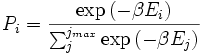
Invoking the concept of the canonical ensemble, it is possible to derive the probability $P_i$ that a macroscopic system in thermal equilibrium with its environment will be in a given microstate with energy $E_i$ :

$P_i = {expleft(-eta E_i ight)over{sum_j^{j_{max}}expleft(-eta E_j ight)}}$

where $eta={1over{kT}}$ ,

The temperature $T$ arises from the fact that the system is in thermal equilibrium with its environment. The probabilities of the various microstates must add to one, and the normalization factor in the denominator is the canonical partition function:

$Z = sum_j^{j_{max}} expleft(-eta E_j ight)$

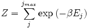
where $E_i$ is the energy of the $i$ th microstate of the system. The partition function is a measure of the number of states accessible to the system at a given temperature. The article canonical ensemble contains a derivation of Boltzmann's factor and the form of the partition function from first principles.

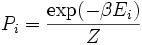
To sum up, the probability of finding a system at temperature $T$ in a particular state with energy $E_i$ is

$P_i = frac{exp(-eta E_i)}{Z}$

[edit]

Thermodynamic Connection

The partition function can be used to find the expected (average) value of any microscopic property of the system, which can then be related to macroscopic variables. For instance, the expected value of the microscopic energy $E$ is interpreted as the microscopic definition of the thermodynamic variable internal energy $U$ ., and can be obtained by taking the derivative of the partition function with respect to the temperature. Indeed,

$langle E angle={sum_i E_i e^{-eta E_i}over Z}=-{dZover deta}/Z$

implies, together with the interpretation of $<E>$ as $U$ , the following microscopic definition of internal energy:

$Ucolon = -{dln Zover d eta}.$

The entropy can be calculated by (see Shannon entropy)

${Sover k} = - sum_i p_i ln p_i = sum_i {e^{-eta E_i}over Z}(eta E_i+ln Z) = ln Z + eta U$

which implies that

$-frac{ln(Z)}{eta} = U - TS = F$

is the Free energy of the system or in other words,

$Z=e^{-eta F},$

Having microscopic expressions for the basic thermodynamic potentials $U$ (internal energy), $S$ (entropy) and $F$ (free energy) is sufficient to derive expressions for other thermodynamic quantities. The basic strategy is as follows. There may be an intensive or extensive quantity that enters explicitly in the expression for the microscopic energy $E_i$ , for instance magnetic field (intensive) or volume (extensive). Then, the conjugate thermodynamic variables are derivatives of the internal energy. The macroscopic magnetization (extensive) is the derivative of $U$ with respect to the (intensive) magnetic field, and the pressure (intensive) is the derivative of $U$ with respect to volume (extensive).

The treatment in this section assumes no exchange of matter (i.e. fixed mass and fixed particle numbers). However, the volume of the system is variable which means the density is also variable.

This probability can be used to find the average value, which corresponds to the macroscopic value, of any property, $J$ , that depends on the energetic state of the system by using the formula:

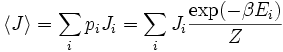
$langle J angle = sum_i p_i J_i = sum_i J_i frac{exp(-eta E_i)}{Z}$

where $<J>$ is the average value of property $J$ . This equation can be applied to the internal energy, $U$ :

$U = sum_i E_i frac{exp(eta E_i)}{Z}$

Subsequently, these equations can be combined with known thermodynamic relationships between $U$ and $V$ to arrive at an expression for pressure in terms of only temperature, volume and the partition function. Similar relationships in terms of the partition function can be derived for other thermodynamic properties as shown in the following table.

Helmholtz free energy:	$F = - {ln Zover eta}$
Internal energy:	$U = -left( frac{partialln Z}{partialeta} ight)_{N,V}$
Pressure:	$P = -left({partial Fover partial V} ight)_{N,T}= {1over eta} left( frac{partial ln Z}{partial V} ight)_{N,T}$
Entropy:	$S = k (ln Z + eta U),$
Gibbs free energy:	$G = F+PV=-{ln Zover eta} + {Vover eta} left( frac{partial ln Z}{partial V} ight)_{N,T}$
Enthalpy:	$H = U + PV,$
Constant Volume Heat capacity:	$C_V = left( frac{partial U}{partial T} ight)_{N,V}$
Constant Pressure Heat capacity:	$C_P = left( frac{partial H}{partial T} ight)_{N,P}$
Chemical potential:	$mu_i = -{1over eta} left( frac{partial ln Z}{partial N_i} ight)_{T,V,N}$

To clarify, this is not a grand canonical ensemble.

It is often useful to consider the energy of a given molecule to be distributed among a number of modes. For example, translational energy refers to that portion of energy associated with the motion of the center of mass of the molecule. Configurational energy refers to that portion of energy associated with the various attractive and repulsive forces between molecules in a system. The other modes are all considered to be internal to each molecule. They include rotational, vibrational, electronic and nuclear modes. If we assume that each mode is independent (a questionable assumption) the total energy can be expressed as the sum of each of the components:

$E = E_t + E_c + E_n + E_e + E_r + E_v,$

Where the subscripts $t$ , $c$ , $n$ , $e$ , $r$ , and $v$ correspond to translational, configurational, nuclear, electronic, rotational and vibrational modes, respectively. The relationship in this equation can be substituted into the very first equation to give:

$Z = sum_i expleft(-eta(E_{ti} + E_{ci} + E_{ni} + E_{ei} + E_{ri} + E_{vi}) ight)$

$= sum_i expleft(-eta E_{ti} ight) expleft(-eta E_{ci} ight) expleft(-eta E_{ni} ight) expleft(-eta E_{ei} ight) expleft(-eta E_{ri} ight) expleft(-eta E_{vi} ight)$

If we can assume all these modes are completely uncoupled and uncorrelated, so all these factors are in a probability sense completely independent, then

$Z = Z_t Z_c Z_n Z_e Z_r Z_v,$

Thus a partition function can be defined for each mode. Simple expressions have been derived relating each of the various modes to various measurable molecular properties, such as the characteristic rotational or vibrational frequencies.

Expressions for the various molecular partition functions are shown in the following table.

Nuclear	$Z_n = 1 qquad (T < 10^8 K)$
Electronic	$Z_e = W_0 exp(kT D_e + W_1 exp(- heta_{e1}/T) + cdots)$
Vibrational	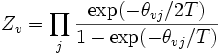$Z_v = prod_j frac{exp(- heta_{vj} / 2T)}{1 - exp(- heta_{vj} / T)}$
Rotational (linear)	$Z_r = frac{T}{sigma} heta_r$
Rotational (non-linear)	$Z_r = frac{1}{sigma}sqrt{frac{{pi}T^3}{ heta_A heta_B heta_C}}$
Translational	$Z_t = frac{(2 pi mkT)^{3/2}}{h^3}$
Configurational (ideal gas)	$Z_c = V,$

These equations can be combined with those in the first table to determine the contribution of a particular energy mode to a thermodynamic property. For example the "rotational pressure" could be determined in this manner. The total pressure could be found by summing the pressure contributions from all of the individual modes, ie:

$P = P_t + P_c + P_n + P_e + P_r + P_v,$

[edit]

Grand canonical ensemble

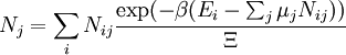
If the system under study is an open system, (matter can be exchanged), and particle number is conserved, we would have to introduce chemical potentials, μ_j, j=1,...,n and replace the canonical partition function with the grand canonical partition function:

$Xi(V,T,mu) = sum_i expleft(eta left[sum_{j=1}^n mu_j N_{ij}-E_i ight ] ight)$

where N_ij is the number of j^th species particles in the i^th configuration. Sometimes, we also have other variables to add to the partition function, one corresponding to each conserved quantity. Most of them, however, can be safely interpreted as chemical potentials. In most condensed matter systems, things are nonrelativistic and mass is conserved. However, most condensed matter systems of interest also conserve particle number approximately (metastably) and the mass (nonrelativistically) is none other than the sum of the number of each type of particle times its mass. Mass is inversely related to density, which is the conjugate variable to pressure. For the rest of this article, we will ignore this complication and pretend chemical potentials don't matter. See grand canonical ensemble.

Let's rework everything using a grand canonical ensemble this time. The volume is left fixed and does not figure in at all in this treatment. As before, j is the index for those particles of species j and i is the index for microstate i:

$U = sum_i E_i frac{exp(-eta (E_i-sum_j mu_j N_{ij}))}{Xi}$

$N_j = sum_i N_{ij} frac{exp(-eta (E_i-sum_j mu_j N_{ij}))}{Xi}$

Gibbs free energy:	$G = - {ln Xiover eta}$
Internal energy:	$U = -left( frac{partialln Xi}{partialeta} ight)_{mu}+sum_i{mu_iovereta}left({partial ln Xiover partial mu_i} ight )_{eta}$
Particle number:	$N_i={1overeta}left({partial ln Xiover partial mu_i} ight)_eta$
Entropy:	$S = k (ln Xi + eta U- eta sum_i mu_i N_i),$
Helmholtz free energy:	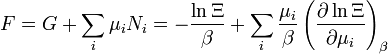$F = G+sum_i mu_i N_i=-{ln Xiover eta} +sum_i{mu_iover eta} left( frac{partial ln Xi}{partial mu_i} ight)_{eta}$

[edit]

Equivalence between descriptions at the thermodynamic limit

All the above descriptions differ in the way they allow the given system to fluctuate between its configurations.

In the micro-canonical ensemble, the system exchanges no energy with the outside world, and is therefore not subject to energy fluctuations, while in the canonical ensemble, the system is free to exchange energy with the outside in the form of heat.

In the thermodynamic limit, which is the limit of large systems, fluctuations become negligible, so that all these descriptions converge to the same description. In other words, the macroscopic behavior of a system does not depend on the particular ensemble used for its description.

Given these considerations, the best ensemble to choose for the calculation of the properties of a macroscopic system is that ensemble which allows the result be most easily derived.

[edit]

Random Walkers

The study of long chain polymers has been a source of problems within the realms of statistical mechanics since about the 1950's. One of the reasons however that scientists were interested in their study is that the equations governing the behaviour of a polymer chain were independent of the chain chemistry. What is more, the governing equation turns out to be a random (diffusive) walk in space. Indeed, Schrodinger's equation is itself a diffusion equation in imaginary time, $t' = i t$ .

[edit]

Random Walks in Time

The first example of a random walk is one in space, whereby a particle undgoes a random motion due to external forces in its surrounding medium. A typical example would be a pollen grain in a beaker of water. If one could somehow "dye" the path the pollen grain has taken, the path observed is defined as a random walk.

Consider a toy problem, of a train moving along a 1D track in the x-direction. Suppose that the train moves either a distance of + or - a fixed distance b, depending on whether a coin lands heads or tails when flipped. Lets start by considering the statistics of the steps the toy train takes:

$langle S_{i} angle = 0$ ; due to a priori equally likely probabilities
$langle S_{i} S_{j} angle = b^2 delta_{ij}$

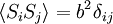
The second quantity is known as the correlation function. The delta is the kronecker delta which tells us that if the indices i and j are different, then the result is 0, but if i = j then the kronecker delta is 1, so the correlation function returns a value of $b 2$ . This makes sense, because if i = j then we are considering the same step. Rather trivially then it can be shown that the average displacement of the train from the x-axis is 0;

$x = sum_{i=1}^{N} S_{i}$
$langle x angle = langle sum_{i=1}^{N} S_{i} angle$
$langle x angle = sum_{i=1}^{N} langle S_{i} angle$

As stated $langle S_{i} angle$ is 0, so the sum of 0 is still 0. It can also be shown, using the same method demonstrated above, to calculate the root mean square value of problem. The result of this calculation is given below

$x_{rms} = sqrt {langle x^2 angle} = b sqrt N$

From the diffusion equation it can be shown that the distance a diffusing particle moves in a media is proportional to the root of the time the system has been diffusing for, where the proportionality constant is the root of the diffusion constant. The above relation, although cosmetically different reveals similar physics, where N is simply the number of steps moved (is loosely connected with time) and b is the characteristic step length. As a consequence we can consider diffusion as a random walk process.

[edit]

Random Walks in Space

Random walks in space can be thought of as snapshots of the path taken by a random walker in time. One such example is the spatial configuration of long chain polymers.

There are two types of random walk in space: Self Avoiding walks, where the links of the polymer chain interact and do not overlap in space, and Pure Random walks, where the links of the polymer chain are non-interacting and links are free to lay on top of one another. The former type is most applicable to physical systems, but their solutions are harder to get at from first principles.

By considering a freely jointed, non-interacting polymer chain, the end-to-end vector is $mathbf{R} = sum_{i=1}^{N} mathbf r_i$ where $mathbf {r}_{i}$ is the vector position of the i-th link in the chain. As a result of the central limit theorem, if N >> 1 then the we expect a Gaussian distribution for the end-to-end vector. We can also make statements of the statistics of the links themselves;
$langle mathbf{r}_{i} angle = 0$ ; by the isotropy of space
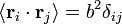$langle mathbf{r}_{i} cdot mathbf{r}_{j} angle = b^2 delta_{ij}$ ; all the links in the chain are uncorrelated with one another
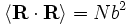Using the statistics of the indivudal links, it is easily shown that $langle mathbf R angle = 0$ and $langle mathbf R cdot mathbf R angle = Nb^2$ . Notice this last result is the same as that found for random walks in time.

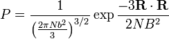
Assuming, as stated, that that distribution of end-to-end vectors for a very large number of identical polymer chains is gaussian, the probability distribution has the following form

$P = frac{1}{left (frac{2 pi N b^2}{3} ight )^{3/2}} exp frac {-3 mathbf R cdot mathbf R}{2NB^2}$

What use is this to us? Recall that according to the principle of equally likely a priori probabilities, the number of microstates, Ω, at some physical value is directly proportional to the probability distribution at that physical value, viz;

$Omega left ( mathbf{R} ight ) = c Pleft ( mathbf{R} ight )$

where c is an arbitrary proportionality constant. Given our distribution function, there is a maxima corresponding to $mathbf {R} = 0$ . Physically this amounts to there being more microstates which have an end-to-end vector of 0 than any other microstate. Now by considering

$S left ( mathbf {R} ight ) = k_B ln Omega {left ( mathbf R ight) }$
$Delta S left( mathbf {R} ight ) = S left( mathbf {R} ight ) - S left (0 ight )$
$Delta F = - T Delta S left ( mathbf {R} ight )$

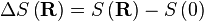
where F is the Helmholtz free energy it is trivial to show that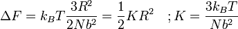

$Delta F = k_B T frac {3R^2}{2Nb^2} = frac {1}{2} K R^2 quad ; K = frac {3 k_B T}{Nb^2}$

A Hookian spring!
This result is known as the Entropic Spring Result and amounts to saying that upon stretching a polymer chain you are doing work on the system to drag it away from its (preferred) equilibrium state. An example of this is a common elastic band, composed of long chain (rubber) polymers. By stretching the elastic band you are doing work on the system and the band behaves like a conventional spring. What is particularly astonishing about this result however, is that the work done in stretching the polymer chain can be related entirely to the change in entropy of the system as a result of the stretching.

[edit]

**A Table of Statistical Mechanics Articles**
	Maxwell Boltzmann	Bose-Einstein	Fermi-Dirac
Particle		Boson	Fermion
Statistics	Partition function Identical particles#Statistical properties Microcanonical ensemble \| Canonical ensemble \| Grand canonical ensemble
Statistics	Maxwell-Boltzmann statistics Maxwell-Boltzmann distribution Boltzmann distribution Derivation of the partition function Gibbs paradox	Bose-Einstein statistics	Fermi-Dirac statistics
Thomas-Fermi approximation	gas in a box gas in a harmonic trap
Gas	Ideal gas	Bose gas Debye model Bose-Einstein condensate Planck's law of black body radiation	Fermi gas Fermion condensate
Chemical Equilibrium	Classical Chemical equilibrium

References

Huang, Kerson (1990). Statistical Mechanics. Wiley, John & Sons, Inc. ISBN 0471815187.
Kroemer, Herbert; Kittel, Charles (1980). Thermal Physics (2nd ed.). W. H. Freeman Company. ISBN 0716710889.

[edit]

External links

Philosophy of Statistical Mechanics article by Lawrence Sklar for the Stanford Encyclopedia of Philosophy.

edit General subfields within physics
Atomic, molecular, and optical physics \| Classical mechanics \| Condensed matter physics \| Continuum mechanics \| Electromagnetism \| Special relativity \| General relativity \| Particle physics \| Quantum field theory \| Quantum mechanics \| Statistical mechanics \| Thermodynamics

سپهر جمعه 26 خرداد‌ماه سال 1385 ساعت 02:08 ب.ظ

0 نظر

دانشنامه آزاد ۴ زبانه / εγκυκλοπαίδεια / licence

دانشنامه آزاد ۴ زبانه / εγκυκλοπαίδεια / licence

درباره من

Contents

Fundamental postulate

Microcanonical ensemble

Canonical ensemble

Thermodynamic Connection

Grand canonical ensemble

Equivalence between descriptions at the thermodynamic limit

Random Walkers

Random Walks in Time

Random Walks in Space

See also

References

External links

دانشنامه آزاد ۴ زبانه / εγκυκλοπαίδεια / licence

درباره من

روزانه‌ها

پیوندها

دسته‌ها

جدیدترین یادداشت‌ها

نویسندگان

بایگانی

Contents

Fundamental postulate

Microcanonical ensemble

Canonical ensemble

Thermodynamic Connection

Grand canonical ensemble

Equivalence between descriptions at the thermodynamic limit

Random Walkers

Random Walks in Time

Random Walks in Space

See also

References

External links